Chapter 2 Setting up R
Welcome to R! For this introductory workshop, we will be using R Markdown. This might take a bit of getting used to it, but it is a great way to run R code and make comments so you know what you did!!
First thing that you will need to do is install the packages you need. The data set, as well as many of the commands is in a library called survival (good name, right!). We will also be using a powerful graphing software called ggplot (boy, we could have up to 5 workshops on this and still only scratch the surface of what this can do!) and a few extra libraries to make things look nice.
First, in the console, you will need to install the packages onto your local drive. To do so, type the commands:
install.packages(“survival”)
install.packages(“ggplot2”)
install.packages(“gridExtra”)
install.packages(“survminer”)
You will only need to do this once. Once they have been installed, you now have them on your local drive.
Now let’s open a new R Markdown notebook. Go to File -> New File -> R Markdown… This will open an R Markdown file for you. Go ahead and run some of the “R Chunks” to see what is going on here. After you are comfortable, let’s change the first chunk to do what we need it to do. We will need to library the survival and ggplot2 package, as well as the other packages we will need. See below for code to do this. Every time you open this document, and want to run the codes contained within, you will need to do these commands first.
library(survival)
library(ggplot2)
library(gridExtra)
library(survminer)
Be sure to hit the little green run button in the right hand corner to run this code. Feel free to put comments before or after this chunk to let you know what you just did!!
Now let’s explore the data set we will be using (as any good data scientist, you must KNOW your data first!!). Go ahead and ask for a summary of the data set lung.
summary(lung)## inst time status age
## Min. : 1.00 Min. : 5.0 Min. :1.000 Min. :39.00
## 1st Qu.: 3.00 1st Qu.: 166.8 1st Qu.:1.000 1st Qu.:56.00
## Median :11.00 Median : 255.5 Median :2.000 Median :63.00
## Mean :11.09 Mean : 305.2 Mean :1.724 Mean :62.45
## 3rd Qu.:16.00 3rd Qu.: 396.5 3rd Qu.:2.000 3rd Qu.:69.00
## Max. :33.00 Max. :1022.0 Max. :2.000 Max. :82.00
## NA's :1
## sex ph.ecog ph.karno pat.karno
## Min. :1.000 Min. :0.0000 Min. : 50.00 Min. : 30.00
## 1st Qu.:1.000 1st Qu.:0.0000 1st Qu.: 75.00 1st Qu.: 70.00
## Median :1.000 Median :1.0000 Median : 80.00 Median : 80.00
## Mean :1.395 Mean :0.9515 Mean : 81.94 Mean : 79.96
## 3rd Qu.:2.000 3rd Qu.:1.0000 3rd Qu.: 90.00 3rd Qu.: 90.00
## Max. :2.000 Max. :3.0000 Max. :100.00 Max. :100.00
## NA's :1 NA's :1 NA's :3
## meal.cal wt.loss
## Min. : 96.0 Min. :-24.000
## 1st Qu.: 635.0 1st Qu.: 0.000
## Median : 975.0 Median : 7.000
## Mean : 928.8 Mean : 9.832
## 3rd Qu.:1150.0 3rd Qu.: 15.750
## Max. :2600.0 Max. : 68.000
## NA's :47 NA's :14You can see how many variables you have, the range of each variable and how many NA’s there are (NA’s can be a problem in some analyses). Let’s take a look at a bar plot for status.
ggplot(lung,aes(x=factor(status)))+ geom_bar(stat="count", fill="blue") Just a little more exploration (if you are doing an analysis, you should explore more than this!).
p1<-ggplot(lung,aes(x=factor(status),y=time)) + geom_boxplot()
p2<-ggplot(lung, aes(x=factor(status),y=age)) + geom_boxplot()
p3<-ggplot(lung, aes(x=factor(status),y=ph.karno)) + geom_boxplot()
p4<-ggplot(lung, aes(x=factor(status),y=pat.karno)) + geom_boxplot()
p5<-ggplot(lung, aes(x=factor(status),y=meal.cal)) + geom_boxplot()
p6<-ggplot(lung, aes(x=factor(status),y=wt.loss)) + geom_boxplot()
grid.arrange(p1, p2, p3, p4, p5, p6, nrow = 3)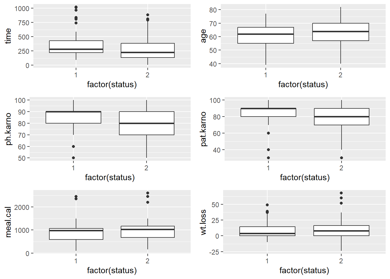
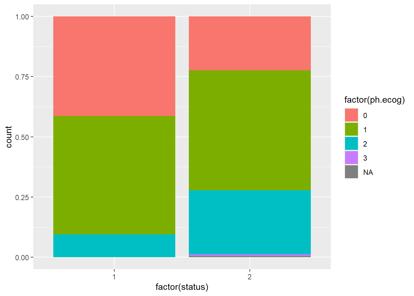
ggplot(lung, aes(x=factor(status),fill = factor(ph.ecog))) +
  geom_bar(position="fill")